How to benchmark your DSP implementations using SNR
In this article I will show an alternative methodology to the default Golden Model approach with bit-true simulations.
If you are looking for the code: github.com/mnemocron/SNR
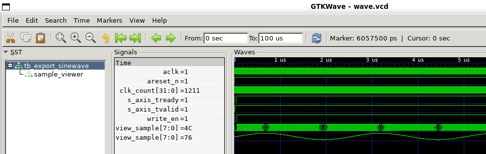 Fig 1: Sine waveform simulated in GHDL.
One often taught way of DSP algorithm design goes something like this:
- Define performance specifications of the algorithm (bandwith, ripple, spectral impurities etc.)
- Draft the required DSP blocks
- Simluate each DSP function in a high-level program (python, matlab)
- Create a bit-true Golden Model with the high-level tool (quantization)
- Implement DSP algorithm with a HDL language
- Simulate HDL model and compare output against Golden Model
I have seen that engineers sometimes skip steps 4. and 6. Instead they are eyeballing the resulting HDL simulation to be good enough.
The suboptimal approach to verify a DSP algorithm in HDL: “If a sine wave goes in and a sine wave comes out, it probably works well enough.”
Frankly, I don’t blame them for this approach.
Writing a solid testbench with assert statements that cover both the exact moment in time and the bit-true vector is challenging enough.
It becomes even more challenging if the algorithm requires small changes like the introduction of pipeline stages to achieve timing closure or the introduction of a resource friendly rounding method.
These type of changes will require a careful inspection of test case evaluation if the testbench is supposed to be self checking.
I propose to merge combine step 6. and 1. In other words, check the output of the HDL simulation against the requirements.
The SNR Funtion in MATLAB
If you have ever developed DSP algorithms in Matlab/Simulink, you must know the handy functions snr(x) and sfdr(x). Both functions are able to take a single argument in the form of an array of samples.
The functions will then calculate either the SNR or SFDR under the assumption that the sampled signal represents a (noisy, distorted) sine wave.
A python script
Shoutout to hrtlacek on Github who recreated the Matlab function in python: github.com/hrtlacek/SNR. I adapted the method for my use case to process binary bit strings from a VHDL simulation output. Fig. 2 shows how the script is used to print a single SNR value of a file that has been written by the VHDL testbench.
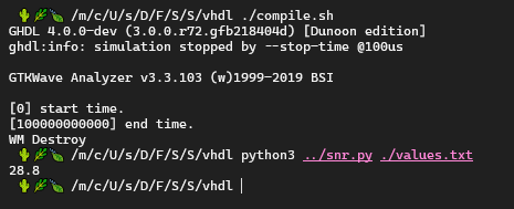 Fig 2: Using the SNR script to calculate the SNR value from a VHDL simulation.
Benchmarking the SNR script
SNR Error: Noise Definition vs. Calculated from Spectrum
The table below lists the error between the definition of the SNR and the calculated SNR in dB. Various noise levels (\(\sigma^2\)) and frequencies (\(\frac{f}{f_S}\)) have been evaluated. There is a maximum error of 0.45 dB.
\[\mathrm{SNR}=\frac{\sigma_\mathrm{signal}^2}{\sigma_\mathrm{noise}^2}\]| 𝜎 [1/Hz] | 0.0001 | 0.001 | 0.005 | 0.01 | 0.02 | 0.05 | 0.1 | 0.2 |
|---|---|---|---|---|---|---|---|---|
| f/fs | ||||||||
| 0.001 | 0.19 | 0.03 | 0.00 | -0.06 | 0.02 | 0.35 | -0.13 | -0.19 |
| 0.01 | -0.15 | -0.01 | -0.20 | 0.01 | 0.16 | 0.10 | -0.14 | 0.33 |
| 0.05 | -0.06 | 0.22 | 0.11 | 0.11 | 0.05 | 0.08 | 0.16 | 0.45 |
| 0.1 | 0.22 | 0.14 | 0.07 | 0.11 | -0.06 | -0.01 | -0.00 | -0.11 |
| 0.2 | -0.05 | 0.08 | -0.01 | 0.12 | 0.19 | -0.00 | 0.01 | 0.38 |
| 0.3 | 0.12 | 0.07 | 0.11 | -0.11 | -0.16 | 0.11 | -0.22 | 0.16 |
| 0.49 | 0.02 | 0.07 | -0.07 | 0.01 | 0.07 | 0.20 | 0.06 | 0.21 |
SNR Calculated from Spectrum: Quantization vs. Frequency
The table below lists the calculated SNR introduced by various degrees of quantization. To calculate the expected SNR, the well known approximation formula \(1.76 + 6.02 \cdot N\) is used.
Here, the calculated SNR shows a greater variance and a dependency of the signal frequency. The errors are sometimes more than 3dB.
| N | 2 | 4 | 8 | 10 | 12 | 14 | 16 | 24 | bit quantization |
|---|---|---|---|---|---|---|---|---|---|
| 13.8 | 25.8 | 49.9 | 61.9 | 74.0 | 86.0 | 98.0 | 146.2 | (1.76 + 6.02 * N) | |
| f/fs | |||||||||
| 0.0001 | 13.8 | 27.8 | 50.8 | 62.7 | 74.8 | 86.8 | 98.7 | 147.1 | |
| 0.001 | 9.7 | 23.6 | 47.8 | 59.7 | 71.9 | 84.0 | 95.8 | 144.1 | |
| 0.01 | 9.9 | 23.9 | 49.1 | 60.7 | 73.5 | 84.2 | 96.1 | 143.7 | |
| 0.1 | 11.3 | 28.0 | 53.0 | 65.1 | 77.1 | 89.2 | 101.2 | 149.4 | |
| 0.25 | 11.0 | 27.8 | 53.0 | 65.1 | 77.2 | 89.2 | 101.2 | 149.4 | |
| 0.3 | 11.4 | 28.1 | 53.0 | 65.1 | 77.1 | 89.2 | 101.2 | 149.4 | |
| 0.49 | 9.1 | 24.3 | 49.4 | 61.2 | 74.0 | 83.9 | 95.5 | 143.7 |
VHDL IEEE.math_real library has a terrible sine implementation
Fig. 1 shows a typical simulation of a waveform in VHDL.
Further down, you will find the VHDL code used to internally generate a sine wave using the VHDL standard library: IEEE.math_real.
Note that this is not syntesizable code but rather a quick signal generator for a testbench.
The testbench then writes the binary bit vectors of width SAMPLE_WIDTH from s_axis_tdata to a text file.
This text file is read by the python script to calculate the SNR.
When I first ran this, I was surprised to read a much worse SNR than expected.
For an N=16 bit quantized signal, the script returns:
- 98.1 dB (python)
- 76.8 dB (VHDL)
  p_wave_stimuli : process
      variable t_pp : real := 0.0;
      variable f : real := 100000.0;
      variable a : real := 0.999;
      variable x : real := 0.0;
      variable sample : std_logic_vector(SAMPLE_WIDTH - 1 downto 0) := (others => '0');
  begin
      wait until areset_n = '1';
      wait until rising_edge(aclk);

      while true loop
          wait until rising_edge(aclk);
          for ii in 0 to N_SAMPLES_PER_TRANSATION - 1 loop
              x := a*sin(2.0 * math_pi * f * t_pp);

              sample := std_logic_vector(to_signed(integer(round(x * (2.0 ** real(SAMPLE_WIDTH - 1) - 1.0))), SAMPLE_WIDTH));
              s_axis_tdata(ii * SAMPLE_WIDTH + SAMPLE_WIDTH - 1 downto ii * SAMPLE_WIDTH) <= sample;

              if areset_n = '0' then
                  t_pp := 0.0;
              elsif s_axis_tready = '1' then
                  t_pp := t_pp + 5.0e-9;  -- CLK_PERIOD
              end if;
              s_axis_tvalid <= '1';
          end loop;
      end loop;
      wait;
  end process;
Something is not right. The SNR script is working correctly for the python generated samples. It has to be the VHDL data. When comparing the waveforms from both implementations, something becomes clear: they are not the same despite being syntesized using the same parameters for frequency, amplitude and quantization. Fig. 3 clearly shows a growing error between the two signals with increasing time. This indicates a frequency offset.
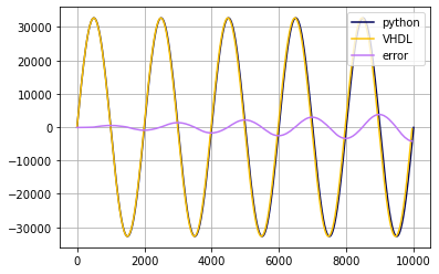 Fig 3: Comparison between sine waves generated from python and VHDL using the same parameters.
With a bit of trial and error I corrected the frequency in python to match the frequency of the signal from VHDL. Another adjustment for the phase was also necessary (\(\phi=0.0032\,\mathrm{rad}\)).
# rebulid the sine wave from the VHDL simulation
CLK_PERIOD = 5e-9
fs = 1/CLK_PERIOD
fu =  100000.0 + 401.0 # + frequency correction
a = 0.999
N = 10000
phi = 0.0032 # phase correction
M = 16
Using those adjusted parameters the resulting error is much smaller and periodic as shown in Fig. 4. And Fig. 5 shows a close up on the small signal error. This is obviously enough to drop the SNR by more than 20dB.
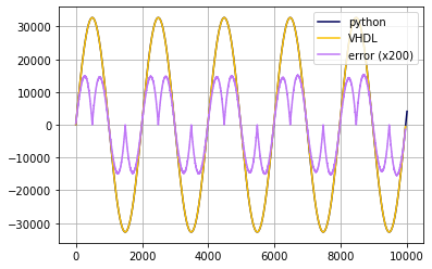 Fig 4: Comparison between sine waves generated in VHDL and adjusted python code.
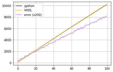 Fig 5: Close up of the error between the two simulations.
I ran the VHDL simulation both in GHDL and Vivado 2024 with the same result.
So far I have not been able to find an explanation for this (I did not actually research it).
If you know more about the sin/cos implementation in IEEE.math_real library I would be happy to hear about it.
In conclusion
Limitations of the SNR script: Because of the limited accuracy with errors ~3dB the script may only detect large systematic errors in the signal processing chain such as interruptions, overflows or large gain errors. An example is shown in Fig. 6.
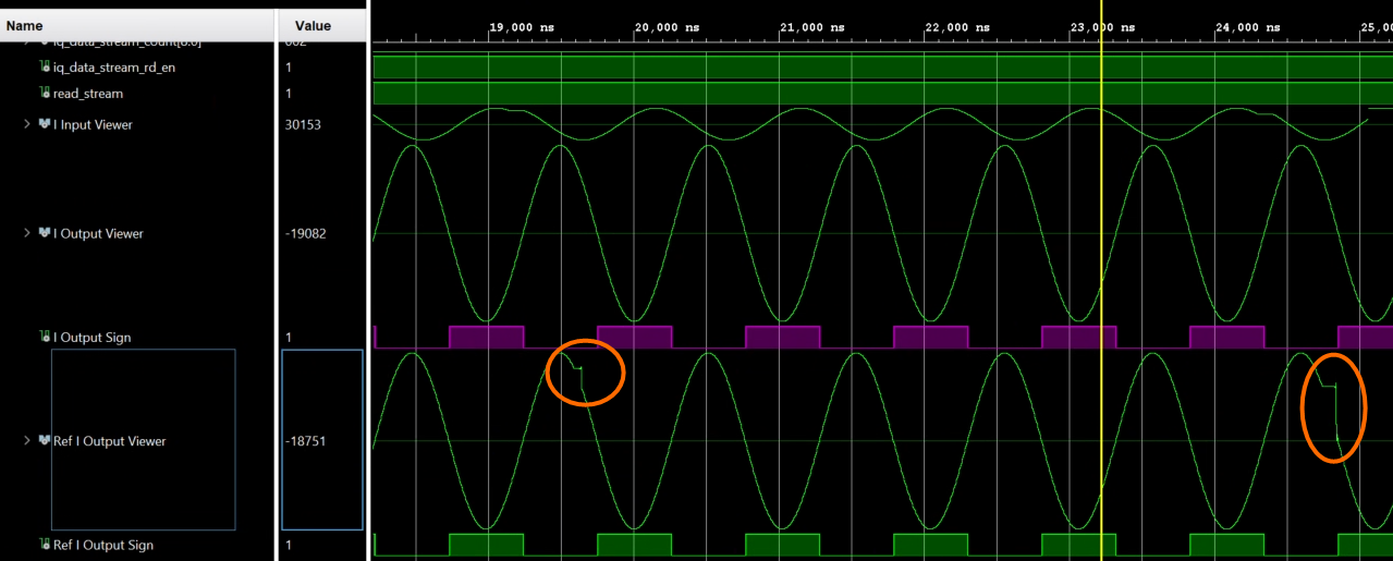 Fig 6: Large errors introduced into the data stream.
In my ideal scenario this script can be implemented in automated tests of a continuous integration (CI) pipeline. This is especially helpful for projects that are continuously worked on to implement new features and add bugfixes. A workflow like this poses a risk of introducing new bugs that break the DSP chain. Here, a unit test for the DSP components can be set up to automatically simulate the DSP entities and generate a waveform file of the output. The SNR script can then calculate the SNR from that simulation and check either for an absolute tolerance in SNR or for a significant change in SNR compared to a different code version.